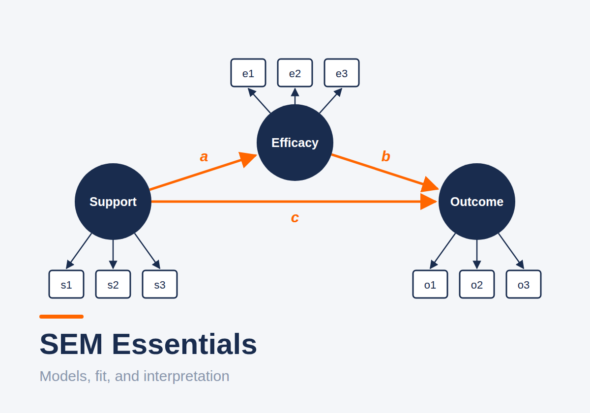
Structural equation modeling (SEM) has a vocabulary problem. Latent variables, identification, modification indices, RMSEA: the words pile up faster than the ideas. Underneath, the ideas are few and very reasonable. This post is the short tour I give people before they open lavaan for the first time.
The two parts of every SEM
An SEM is two models stacked together:
- The measurement model says how latent variables (constructs you cannot observe directly) show up in observed indicators. This is a confirmatory factor analysis (CFA): each item is a function of a factor plus error.
- The structural model says how the latent variables relate to each other: regressions, correlations, indirect effects.
Path analysis is the special case with no latent variables, just observed ones. CFA is the special case with only a measurement model. Full SEM is both.
The big payoff is error. Because constructs are measured by several indicators, the structural paths are estimated between the error-free parts of the constructs. Regression on sum scores cannot do that, which is why it tends to underestimate relationships.
Identification: can the model be estimated at all?
A model is identified if its parameters can be uniquely recovered from the covariance matrix (and means, if you model them). Three habits cover most cases:
- Count. With p observed variables you have p(p + 1)/2 unique variances and covariances. You need at least as many as free parameters. The difference is your degrees of freedom.
- Set a scale for each latent variable. Either fix one loading to 1 (marker variable, lavaan's default) or fix the factor variance to 1. Same fit, different metric.
- Watch small factors. A factor with only two indicators is identified only if it correlates with other factors. Three or more indicators per factor keeps life simple.
Estimation: pick the estimator that matches the data
- ML: continuous, roughly normal indicators.
- MLR: continuous but non-normal data. Robust standard errors and a scaled test statistic. Also handles missing data through full-information ML.
- WLSMV: ordinal indicators (Likert items with few categories, binary items). Treating five-point items as continuous is often fine with five or more categories, but less so with skew or fewer categories.
The estimator is not a detail for the appendix. It changes standard errors, fit statistics, and sometimes conclusions.
Fit: how well does the model reproduce the data?
Fit indices compare the covariance matrix implied by your model with the observed one.
- χ² test: an exact-fit test. Useful, but with large samples it rejects almost every model for trivial misfit.
- CFI / TLI: how much better your model is than a model where nothing correlates. Closer to 1 is better.
- RMSEA: misfit per degree of freedom, with a confidence interval. Closer to 0 is better.
- SRMR: the average standardized residual correlation. Closer to 0 is better.
The Hu and Bentler (1999) cutoffs (CFI around .95, RMSEA around .06, SRMR around .08) are everywhere, but they came from a specific set of simulation conditions and were never meant as universal pass/fail lines. Treat them as a rough compass. Then look at the local fit: residual correlations tell you where a model is wrong, which global indices never do.
And resist the modification index slot machine. I wrote a whole post on that: SEM Without Fit-Chasing.
Interpretation: reading the output
- Unstandardized estimates are in the units of your variables. Use them when units mean something.
- Standardized estimates put everything in standard deviation units. Loadings become item-factor correlations (for simple structure), and structural paths become comparable across predictors.
- R² for each indicator is the share of its variance explained by the factor. Low values point to weak items.
- Indirect effects are products of paths. Their sampling distributions are skewed, so use bootstrap confidence intervals rather than the normal-theory standard error.
Quick R sketch (lavaan)
library(lavaan)

model <- '
  # measurement model
  support  =~ s1 + s2 + s3
  efficacy =~ e1 + e2 + e3
  outcome  =~ o1 + o2 + o3

  # structural model
  efficacy ~ a * support
  outcome  ~ b * efficacy + c * support

  # indirect and total effects
  indirect := a * b
  total    := c + a * b
'

fit <- sem(model, data = dat, estimator = "MLR", missing = "fiml")
summary(fit, fit.measures = TRUE, standardized = TRUE, rsquare = TRUE)

# local fit: residual correlations above |.10| deserve a look
resid(fit, type = "cor")

# bootstrap CI for the indirect effect
fit_boot <- sem(model, data = dat, se = "bootstrap", bootstrap = 2000)
parameterEstimates(fit_boot, boot.ci.type = "perc")
A short checklist
- Draw the model before you touch the data.
- Check identification and degrees of freedom.
- Choose the estimator from the data type, not from habit.
- Fit the measurement model first. Fix measurement problems before adding structure.
- Report global fit, local fit, and every change you made along the way.
- Interpret estimates in the metric that matters for your question.
Closing
SEM is not a fancier regression. It is a way of writing down what you think is going on, including how imperfectly you measure it, and then checking that story against data. Get the essentials right and the rest of the vocabulary starts to feel like detail.
- Fatih